Temporal Pooling Mechanism
In which I implement a temporal pooling mechanism and test it with fancy statistics, only to realise a more fundamental problem: my sequence memory algorithm isn’t predicting mixed sequences well enough (which is a prerequisite to temporal pooling over them).
A central idea in Hierarchical Temporal Memory is that activity in the cortex becomes more stable as one looks further up in the hierarchy of cortical regions. Taking vision as an example, the first regions respond to small parts of the retina and change rapidly. Higher regions will have stable representations of, say, an elephant as we look at it from any angle. This process of abstracting up the hierarchy is referred to as temporal pooling. You can read Jeff Hawkins’ new ideas about temporal pooling.
There should be specific cells which become active in response to, say, an elephant and not for anything else. We can measure this on labelled input data with standard classification metrics. Given a candidate cell:
-
Sensitivity is the fraction of elephant observations on which the cell was (correctly) active.
-
Specificity is the fraction of non-elephant observations on which the cell was (correctly) inactive.
-
Precision is the fraction of the cell’s activations on which an elephant was in fact being observed.
I have attempted to implement a mechanism for temporal pooling. For now, the implementation does not cover the full sensori-motor scheme (only Layer 3 not Layer 4), so the experiments I describe here use only sensory inputs.
Mechanism
EDIT: this idea was first articulated by Jake Bruce.
My mechanism extends the standard spatial pooling (also known as pattern memory), selecting which columns in a region become active. The input data are the active cells from the region below, as well as the subset of those correctly predicted by the region below, which I call signal cells. My mechanism sets up persistent temporal pooling scores which are used like column overlap scores (i.e. to select active columns). Temporal pooling scores are generated for a column when it overlaps with signal cell inputs; they decay over time; they are interrupted when dominated by other columns’ overlap scores, or when bursting (non-signal) input comes in to the column itself.
Notice that I do not explicitly turn off pooling when bursting inputs appear nearby. Rather I assume that bursting inputs will generate dominant overlap scores because bursting column activation is dense compared to the sparse (one cell per column) activation from predicted columns. Whether that is a reasonable assumption in general remains to be seen. Further insights from the biology may help to clarify it. Anyway, the mechanism step-by-step:
-
The overlap score of each column with the input is computed as usual, but any existing temporal pooling scores (see step 5) replace the current overlap scores. code
-
The set of active columns is derived from overlap scores as usual by lateral inhibition. Any columns which did not become active lose their temporal pooling status. code
-
If any column has a current overlap score above its previous temporal pooling score, the previous temporal pooling score is deleted. However, the column may remain in a temporal pooling state if the new overlap comes from signal cells (step 5). code
-
Temporal pooling scores on continuing active columns are reduced by a decay factor. code
-
If any active columns overlap with signal-cell inputs this overlap is multiplied by a signal boosting factor and becomes the column’s new temporal pooling score. code
-
(Sequence Memory / Temporal Memory): In continuing temporal pooling columns, the previously active cell remains active. code In newly active temporal pooling columns, a cell is chosen to become the active temporal pooling cell in the usual way (depending on whether the column itself is bursting or predicted).
-
The temporal pooling cell is active and thus learns by growing lateral synapses. code
See it run
To test my mechanism, I made an input stream consisting of six fixed one-dimensional sequences, each repeating at random intervals, mixed together. See section The data below. You can run it online and observe temporal pooling in the higher region after about 300 time steps:
Sequences mixed with variable gaps
Note: Maximise browser window before loading page. Google Chrome browser recommended.
In the visualisation, columns are coloured as follows:
- red columns are bursting (active without being predicted);
- blue columns had predicted cells but did not become active;
- purple columns were simultaneously active and predicted;
- green columns are in a temporal pooling state and thus are remaining active over multiple time steps. (May be green or brown according to whether the column is itself predicted or bursting).
This screenshot gives an example of temporal pooling:
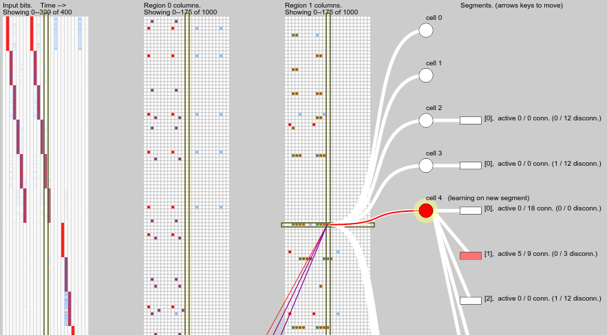
The block on the left shows the input bits, arranged in time steps from left to right. The middle block shows columns of the first region, in corresponding time steps from left to right. Yes it is confusing that the “columns” (neural minicolumns) of a region are themselves arranged in a column (tabular column) for this visualisation. The next block shows columns of the second region, which receives as input the active cells from the first region. One time step is highlighted across all panels, and one column is selected in the highest region, showing its constituent cells and their distal dendrite segments.
The input shows a simple repeated pattern over 6 time steps. The first time step was not predicted since it occurs randomly, but the following 5 time steps were predicted, as indicated by the purple columns in the first region in those time steps. (Later steps of the sequence occur further down in the input field, activating columns further down in the region, so they are not visible here). Predictive columns are also mapped back onto the input bits so we can see which part of the input field was predicted.
The correctly predicted columns in the first region generate temporal pooling scores in the next region, visible as green and brown columns. While the input sequence is correctly predicted, some of these temporal pooling cells remain active.
But let’s try to measure this.
Measurement
To measure the sensitivity, specificity and precision of temporal pooling over a given input pattern, we need to come up with some candidate cells. I did this by “warming up” the system for 5000 time steps, then keeping the following 2000 time steps. I filtered them down to where the given pattern occurs (excluding the first step it appears on, which is unpredictable), and selected the top 3 most frequently active temporal pooling cells. These are my candidates.
It is then a simple matter to compute sensitivity, specificity and precision for each candidate cell. The results are shown in the following table and plot.
| pattern | candidate | in-steps | out-steps | active-in | active-out | sensitivity | specificity | precision |
|---|---|---|---|---|---|---|---|---|
| run-0-5 | 0 | 230 | 1724 | 112 | 27 | 0.49 | 0.98 | 0.81 |
| run-0-5 | 1 | 230 | 1724 | 123 | 46 | 0.53 | 0.97 | 0.73 |
| run-0-5 | 2 | 230 | 1724 | 108 | 21 | 0.47 | 0.99 | 0.84 |
| rev-5-1 | 0 | 192 | 1760 | 109 | 76 | 0.57 | 0.96 | 0.59 |
| rev-5-1 | 1 | 192 | 1760 | 99 | 50 | 0.52 | 0.97 | 0.66 |
| rev-5-1 | 2 | 192 | 1760 | 91 | 17 | 0.47 | 0.99 | 0.84 |
| run-6-10 | 0 | 204 | 1745 | 116 | 151 | 0.57 | 0.91 | 0.43 |
| run-6-10 | 1 | 204 | 1745 | 114 | 115 | 0.56 | 0.93 | 0.50 |
| run-6-10 | 2 | 204 | 1745 | 111 | 133 | 0.54 | 0.92 | 0.45 |
| jump-6-12 | 0 | 204 | 1745 | 117 | 128 | 0.57 | 0.93 | 0.48 |
| jump-6-12 | 1 | 204 | 1745 | 120 | 149 | 0.59 | 0.91 | 0.45 |
| jump-6-12 | 2 | 204 | 1745 | 113 | 151 | 0.55 | 0.91 | 0.43 |
| twos | 0 | 280 | 1680 | 101 | 11 | 0.36 | 0.99 | 0.90 |
| twos | 1 | 280 | 1680 | 89 | 4 | 0.32 | 1.00 | 0.96 |
| twos | 2 | 280 | 1680 | 101 | 44 | 0.36 | 0.97 | 0.70 |
| saw-10-15 | 0 | 268 | 1694 | 157 | 112 | 0.59 | 0.93 | 0.58 |
| saw-10-15 | 1 | 268 | 1694 | 148 | 88 | 0.55 | 0.95 | 0.63 |
| saw-10-15 | 2 | 268 | 1694 | 138 | 76 | 0.51 | 0.96 | 0.64 |
The results are disappointing. While the specificity is reasonably high, sensitivity is low—under 60%—meaning that none of the candidate cells can reliably indicate the presence of its pattern on its own.
ad-lib hypotheses
-
The visual display suggested that cells were indeed staying active over any one pattern instance, but not necessarily the same cells for different instances. So the selection of active columns in the higher region may not be consistent across instances of the pattern.
-
Perhaps this is all we should expect from one region and we should look at an even higher region for more complete temporal pooling.
-
Perhaps the feed-forward synapses are continuing to learn and change and this is causing the inconsistency in column activation. Specifically it may be the learning on temporal pooling columns that is weakening their receptive field.
-
Perhaps feed-forward synapses should be reinforced more strongly when they carry input from signal cells, to make it more likely for those columns to become active again. (I got this idea from nupic.research.)
-
Perhaps column activation should be biased by predicted (depolarised) cells in the column. (I got this idea from Fergal Byrne.) This seems to promise more consistent column activations, rather than the current approach of randomly choosing between any columns with equal receptive field overlaps.
Consistency between pattern instances
Is the problem just randomness in the choice of active colums when each pattern instance appears? If so then I would expect if we looked over a few candidate cells then collectively they would cover all instances of the pattern.
Since I am concerned with the sensitivity measure, I filtered the time steps down to just those where the pattern is occuring, grouped into each instance of its occurence. Below is a plot of activations over time of 25 candidate cells, being the top ones by overall sensitivity. I did this for three different patterns.
The picture is not what I expected. Different candidate cells do not seem to be complementary in their activations, they seem remarkably similar. Some pattern instances see widespread pooling while others do not see pooling at all (i.e. if you look down one bar in the plot, there are no horizontal lines indicating pooling). This suggests that the problem is not spatial pooling (selection of columns) but rather sequence memory (prediction of sequences).
I’d better check this out…
Observing carefully
Hi again. I’ve just been watching the simulation more carefully. Well, now I feel foolish—I see what is going wrong and it is more fundamental than any of the hypotheses I threw up above. The first region is just not predicting the input sequences well in many instances, so of course they are not being pooled over.
While pattern instances that appear in isolation are generally fully predicted, when two patterns occur together the predictions seem to fail.
Take this example, after a generous training period of 4000 time
steps. Four pattern instances are visible (rev-5-1, run-0-5,
jump-6-12, run-6-10), and all but the third have interference
problems.
The clearest case is the last pattern: its initial time step is predicted based on the final step of the previous pattern; but this is a spurious prediction since its occurence is random. So, only one cell per column is active instead of the usual full bursting, and it is evidently not the one that usually predicts the next step of the pattern. The next step appears unexpectedly and bursts the columns. After that the sequence prediction recovers. This suggests that failing predictions should be more harshly punished?
The first pattern is missed on its final timestep, probably due to the mixed input on the second-last time step activating different columns from the ones which usually predict the final time step. This suggests that columns should be preferentially activated if they contain predictive cells?
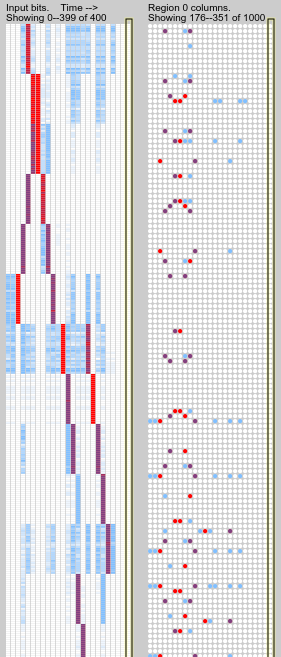
A different kind of prediction failure is shown in the screenshot below. The pattern sequence prediction breaks down after correctly predicting the first 4 time steps. Inspecting the dendrite segments shown we can see there is one that has fallen just below the activation threshold (it has an activation level of 8 and the threshold is 9). This would have been caused by prior incorrect predictions being punished, i.e. the segment synapses being weakened. This suggests that failing predictions should be less harshly punished??

The curse of parametricality
I’ll need to go back to the basic algorithm and confront the many implementation details and parameter values I have chosen. For reference here are the parameter values I used in the simulations described above. You can also view and modify them in the online simulation.
(def spec
  {:ncol 1000
   :potential-radius-frac 0.1
   :activation-level 0.02
   :global-inhibition false
   :stimulus-threshold 3
   :sp-perm-inc 0.05
   :sp-perm-dec 0.01
   :sp-perm-signal-inc 0.05
   :sp-perm-connected 0.20
   :duty-cycle-period 100000
   :max-boost 2.0
   ;; sequence memory:
   :depth 8
   :max-segments 5
   :max-synapse-count 18
   :new-synapse-count 12
   :activation-threshold 9
   :min-threshold 7
   :connected-perm 0.20
   :initial-perm 0.16
   :permanence-inc 0.05
   :permanence-dec 0.01
   })
The code
The demo here was compiled from Comportex 0.0.2 with ComportexViz 0.0.2.
The extra analysis code is here: temporal_pooling_experiments.clj.
The data
The (toy) problem domain I have constructed here is an attempt to test temporal pooling and sequence memory in a simple but meaningful way. I would like others to try simulating the same problem domain, or to suggest any other that can serve as a kind of benchmark or shared example.
The input is made up from 6 different fixed patterns, named as follows:
run-0-5 |
[0 1 2 3 4 5] |
rev-5-1 |
[5 4 3 2 1] |
run-6-10 |
[6 7 8 9 10] |
jump-6-12 |
[6 7 8 11 12] |
twos |
[0 2 4 6 8 10 12 14] |
saw-10-15 |
[10 12 11 13 12 14 13 15] |
These patterns are fed into the input stream, each instance separated from its next repeat by a gap with random duration of between 1 and 75 time steps. As such, the input on each timestep is a set of (up to 6) integers in the range [0 15]. These are encoded by simply dividing up the input array (of 400 bits) into 16 non-overlapping blocks and activating the block corresponding to the integer. The encoded bits from each integer are ORed together. The code is mixed_gaps_1d.cljx.
I have generated a CSV data file containing 10,000 time steps of the input stream: mixed_fixed_1d_10k.csv (70kb).
The file has 6 columns containing either integers or blanks. The set of integers from each row should be encoded with a scalar encoder of range [0 15], bit width 400, and 25 active bits. The final input set is the union of the active bits from each encoded integer.
Thanks for reading this. I would appreciate your advice.
–Felix
P.S. I’m loving charting with variancecharts.com.