The taming of the SDR
In which I come to a way of visually understanding the activity of cells in HTM, which have Sparse Distributed Representations (SDRs). This new way is like a state transition diagram, but with fuzzy, evolving states. Several problems in my existing demos become immediately obvious.
Sparse Distributed Representations
Does the brain work like a computer program? No, and perhaps the deepest explanation of the difference is in their representation of information. Computers store data and instructions in a precise structure using every bit; in a digital memory address, one bad bit makes the whole thing useless. Brains use a sparse, distributed representation where vastly more bits (cells) are needed, but in its own form captures meaning, in terms of a “halo” of related concepts. Read more.
Think of representing a particular person. A computer program might use their name or email address. But that in itself doesn’t tell you anything about the person, and if any bit was wrong it would fail. In contrast, a sparse distributed representation might include where they live, their friends, occupation, etc. If bits of that were missing, one would still have a general idea who it might be or could fall back to someone “similar”.
The problem with using SDRs is that they are hard to pin down. How do you work with something that is:
- fuzzy – it can be active to varying degrees, mixed with noise or other SDRs;
- evolving – it can change over time as it is learned from experience.
A sketch of a diagram
Earlier this year, Rob Freeman and I were exchanging emails on some HTM-related ideas. At one point he said,
I want to experiment with allowing distal excitation to spread over region-1 independently of time steps (or before each time step?)
For instance, if you take my earlier example
abcabcabcxyzabcand plot all the subnetworks in a pooled representation […] it should look like (if my ascii art works out):abc / \ abc - abc \ / xyz
Well, I may have missed the main point Rob was making at the time, but that little ascii-art diagram got me thinking. Why can’t we distil the activity in a HTM region down into a state transition diagram?
I spent the next couple of months, on and off, building and refining such a plot. In retrospect it seems like an obvious visualisation, and I’ve come to rely on it as an essential tool for understanding HTM activity.
The method
I’m going to talk about SDRs of cell activity in a single layer of a HTM network. Note, cell activity, not column activity, which means that these representations are context-specific. And because my main display in ComportexViz shows column activity, it doesn’t help much with seeing these context-specific cell SDRs.
This is as much an algorithm as it is a plot.
The main idea is to tame SDRs by recording them with a unique name when they appear in distinguishable form. Then we can recognise them when they appear again, even partially, and we can decide how to evolve their form.
Let’s call a named SDR a state (since it will play a role on something like a state transition diagram). A state keeps track of which cells have been active on its watch, and how often.
Every time step we check the set of active learning cells. If they overlap a known state sufficiently well, meeting a threshold parameter, that known state is said to match. It’s even possible that multiple states could match. Otherwise, the active learning cells define a new state. In any case, all these cells are counted towards the matching state (or states).
It’s not quite that simple because states are fuzzy. Some cells are more essential to a state than others. That’s why we keep running counts: the influence of a cell is weighted by its specificity to a state. So if a cell participates in states A and B an equal number of times, it will count only half as much to A as a cell fully specific to A. Code.
Here we see there is a tension at the heart of the idea. When a state evolves and expands, as it appears mixed in various different contexts, is it still reasonable to think of it as a single coherent thing? Well, perhaps not, and it will often make sense to reset, building states anew after some time. But abstraction of concepts from fuzzy, messy reality is how we understand the world.
Labels from the input data are also counted on matching states, but this is only for display, it is not used to define states in any way.
So that’s basically it for taming SDRs. Now for the display, at one point in time. We can draw the states, but what about the transitions between them? Those we can derive from distal synapse connections. Easy: get all connections between cells, then map both the source and target cells into states, weighted by specificity. You end up with the connections between states, each with a score, being the weighted number of connected synapses between them. Code.
As well as drawing the matching states, it’s useful to show any partial matches of states by currently active or predicted cells.
Reading the diagram
Here’s an example where the inputs are single letters. This display shows the activity in a layer of cells after seeing the sequence*:
o n e o n e o n e t w o t w o t w o t h r e e
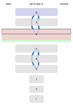
What does it tell us? Firstly, each of the letters of “one” and “two” generated distinct states when they were first seen, were re-activated on repetition, and the transitions between them were learned (blue lines). The start of “three”, “thr” also generated new states, but the “e” matched the previous “e” state from “one” instead of generating a new state. Incidentally, this is undesirable and indicates some bad parameters in this particular example. The current state, at the time this plot was drawn, was matching that “e” state (outlined black), and also extending it with other current cells that were not already in the state (the green part). Lastly, the initial “o” state is being predicted for the next time step (it is shaded blue).
More precisely, here are the rules:
- States are drawn in order of appearance, by default.
- If any of a state’s cells are currently active that fraction will be shaded red (whether active due to bursting or not).
- Similarly, any predictive cells (predicting activation for the next time step) will be shaded blue.
- If any of a state’s cells are the current learning cells that fraction will be outlined in black.
- When a matching state will be extended to include new cells, those are shown in green.
- Transitions are drawn as blue curves. Thickness corresponds to the number of connected synapses, weighted by specificity of both the source and target cells.
- The height of a state corresponds to the (weighted) number of cells it represents.
- The width of a state corresponds to the number of times it has matched.
- Labels are drawn with horizonal spacing by frequency.
Putting it to work
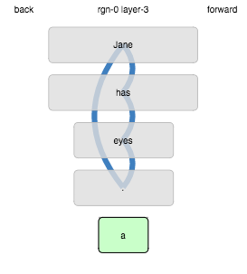
Let’s see if the display is useful. Continuing the example from a previous post we’ll use the following sequence of words as input (with each sentence repeated).
Jane has eyes .
Jane has a head .
Jane has a mouth .
Jane has a brain .
Jane has a book .
Jane has no friend .
Chifung has eyes .
Chifung has a head .
Chifung has a mouth .
Chifung has a brain .
Chifung has no book .
Chifung has a friend .
Here we go.
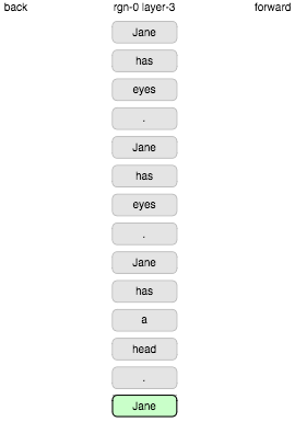
Erm… ok. That’s not good. Every word seen comes up as a completely new state, even when repeated. The problem here was the “boosting” mechanism which is supposed to encourage fair, efficient use of columns by biasing activation towards neglected columns. It does settle down after a while but clearly this is pretty crazy. Let’s turn off boosting.
Running it again, repeated states are now re-activated, but we have a
new problem. Here are two consecutive time steps (has, a):
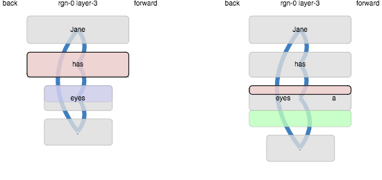
The sequence Jane has eyes had already been learned, so “eyes” was
predicted. When the actual input “a” appeared, it somehow ended up
matching the state that was previously active for “eyes”. How?
The answer is that the predicted cells, with their distal excitation, were biased to become active, so the prediction became part of the actual representation. This is a non-standard part of the algorithm, sometimes called prediction-assisted recognition. However in this case the effect is clearly too strong. We can confirm the cause by looking at the sources of excitation on activated cells:
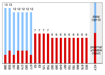
So indeed there were 7 cells which became active on the strength of their predictive (distal) excitation without having much direct (proximal) excitation.
When we revise the parameter :distal-vs-proxmal-weight down from 1.0
to 0.2, the confusion we observed is resolved:
Moving on… when we let it run through, something odd happens in the second section:
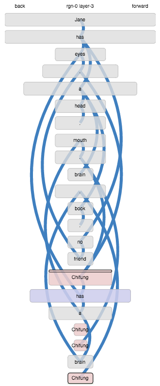
The word “Chifung” ends up as a different state within each
sentence. This happens because, the whole input being an unbroken
sequence, “Chifung” appears after sequences that were recognised
from previous learning:
has no friend . Chifunghas eyes . Chifunghas a head . Chifunghas a brain . Chifung
Coming up in these different learned contexts leads to distinct
context-dependent representations. That feels frustrating, because it
is obvious to us that those are not meaningful contexts, and do not
alter the meaning of “Chifung”.
A better way to read sentences may be using multiple layers. A lower layer learns sequences of words in a sentence, but starts anew rather than continuing sequences across sentence boundaries. A higher layer could track transitions across sentences, which of course involves Temporal Pooling, a topic I won’t discuss here. This approach can be seen in the second-level motor online demo.
There are several online demos at http://nupic-community.github.io/comportexviz/
Looking forward to hearing your thoughts directly or on the NuPIC-theory mailing list.
–Felix
UPDATE 2015-09-18: Chetan, replying on NuPIC-theory, suggested running a higher-order sequence like
6874230
1874235
This is “higher-order” because it’s not enough to learn the transitions in isolation. The context of the first letter must be carried through the following 5 steps in order to unambiguously predict the final letter.
I ran it through my second-level motor demo, where each word is repeated until it is learned before moving on, and the sequence learning is reset when starting each new word. Learning follows a pattern where on each repetition the new pattern becomes progressively more distinct from the old pattern, until after about 6 repetitions there is a fully distinct representation of the new pattern.
You can run this yourself online, but I also recorded it as a video, in case that is easier.
Code
The results here were produced with Comportex 0.0.10 with ComportexViz 0.0.10.
* The first example comes from the second-level motor demo, so the input is not actually a simple sequence.