Attempting the Numenta Anomaly Benchmark
Being an objective test problem, NAB allows us to tease apart the contribution of various aspects of HTM models. It turns out the current best result on NAB can be achieved with only first-order transition memory. It seems the regular sampling rate of most time series data does not produce a directly meaningful sequence of transitions. If we take effective time steps only when sufficient changes occur this indeed gives some improved performance, but still sees no benefit to higher-order transitions. Ultimately, like most things in HTM, I think human-level anomaly detection will require robust temporal pooling.
The most frustrating thing about working on Hierarchical Temporal Memory has been the lack of any standard test problems. I’ve spent ages thinking and reading papers, trying to decide what kind of problems are suitable. Visual object recognition – or does that depend on understanding attention? Game playing – or does that require complex behaviour generation? Natural language processing – or does that need working memory? What even should an HTM system be trying to do and how can we measure it?
To its credit, Numenta has recently established one such standardised test problem: Numenta Anomaly Benchmark (NAB). The task is anomaly detection in a stream of numeric values. It includes a corpus of artificial data, events with known causes, and other real world data annotated with anomalies, each over a window of time. Currently there are 58 time series with a total of about 366,000 records and 116 anomaly windows.
Initial results have an HTM model coming out on top compared with several other methods. This is exciting because it is the first example I have seen of HTM doing something useful, and doing it better than the alternatives.
The HTM model listed on the NAB leaderboard was run in NuPIC with these parameter values. I set out to find out which aspects of the model were really important, by exploring the parameter space and algorithm variations. Also, since at last we have a standard test problem, this was an opportunity to verify my implementation of HTM, Comportex.
Headline result
I have not produced a much better score than the original Numenta model. Rather, my main result was to show that that score can be equalled with a much simpler model. This tells us something useful about the contribution of different aspects of these HTM models. I’ll discuss some below.
The headline result here comes from Comportex with mostly the same parameters as the Numenta model, but with the following differences:
- first-order transition memory (1 cell per column, down from 32);
- a potential receptive field sample of 16% (down from 80%);
- only 16 segments per cell (down from 128);
- sampled linear encoders;
- timestamp given as distal input (not proximal / driving input);
- a distal stimulus threshold of 18 (not 20).
If you’ve been following the HTM community you’ll recognise that this approach is based directly on the successful work of Marcus Lewis.
Additionally, some post-processing was applied:
- Instead of the raw bursting rate, a delta anomaly score was calculated: it considers only newly active columns (ignoring any remaining active from the previous timestep). The bursting rate is calculated only within these new columns. To handle small changes, the number of columns considered – i.e. divided by – is kept from falling below 20% of the total number of active columns (20% of 40 = 8).
- If an anomaly is detected (above some specified threshold), no further detections are reported for 40 time steps. This stops false positives from going crazy.
- Note that Numenta’s Anomaly Likelihood filtering was not applied.
Anyway, here is the final result as scored by NAB:
| model | standard | low FP rate | low FN rate |
|---|---|---|---|
| original NuPIC model + anomaly likelihood | 65.3 | 58.6 | 69.4 |
| original NuPIC model, raw bursting score | 52.5 | 41.1 | 58.3 |
| selected Comportex model, delta anomaly score | 64.6 | 58.8 | 69.6 |
| selected Comportex model, raw bursting score | 59.5 | 53.4 | 63.8 |
A model variant that achieves a notably better low FP rate score of 59.8 is also described below under Effective time steps.
Discussion
This is a good result and confirms that Comportex is a competitive implementation of HTM. But the most interesting part is how this allows us to run experiments to tease apart the contribution of different aspects of the models. Let look at the most important ones:
First-order
The result shows that the reported performance of HTM on NAB can be explained with only first-order transition memory. That is surprising, given that NAB consists of many complex time series, and some were even deliberately constructed as artificial higher-order sequence problems. However, the result follows similar findings for prediction on the HotGym data (by Marcus Lewis), and on the New York Taxi data (by me).
Of course I did run experiments with 32 cells per column, the NuPIC standard. The result was a large decrease in score – around the same amount as when leaving out the timestamp input, or when leaving out the delta anomaly score. (see Appendix)
That a first-order model gives an improved result suggests that the current design of HTM transition memory is incomplete. While it is possible that my own implementation has subtle problems, the fact remains that HTM’s higher order transition memory has not been demonstrated to have a benefit on any real problem, as far as I know. My feeling is that transition memory will work better when constrained by higher-level contexts, i.e. with temporal pooling.
Delta anomaly score
The delta anomaly score is defined as:
(number-of-newly-active-columns-that-are-bursting) /
max(0.2 * number-of-active-columns, number-of-newly-active-columns)
Note that this will not pick up cases when columns stay on
unexpectedly, like a flat-line scenario. To catch this I also tried a
variant with instead the number-of-newly-bursting-columns –
i.e. counting the columns that changed into a bursting state, even if
they were previously active. However, that gave worse results.
Here’s an example of an obvious anomaly in the
realKnownCause/machine_temperature_system_failure series, around
time step 4000:
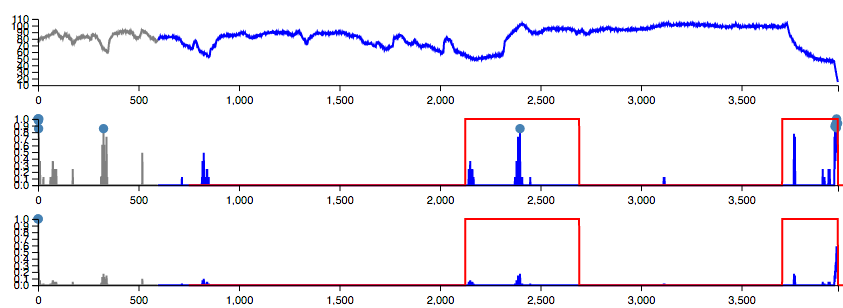
Section of the machine_temperature_system_failure data. Anomaly
windows are outlined in red. The middle plot is delta anomaly scores
and the bottom plot is raw bursting scores, from a baseline HTM
model.
Looking at the HTM columns with Sanity, we can see that the anomaly rolls in over several time steps, hiding the overall magnitude of the anomaly:
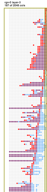
HTM columns over time (time steps go left to right) on the machine_temperature_system_failure data, highlighting time step 3982. Red columns are bursting.
That is why delta anomaly calculation helps. I like that this simple approach achieves good results without the need for a separate “anomaly likelihood” Gaussian estimation process.
Limited potential receptive field
It is curious that there is such a strong benefit in limiting the set of inputs that each column can connect to. I think this reflects that the learning process in HTM is too greedy, so it loses the ability to discriminate between values. A “boosting” mechanism is supposed to correct for this, but in practice does more harm than good. There is more to say on this but I’ll leave that for another time and a simpler test problem.
Compared to the roughly 5% increase in score going from 80% to 16% global connectivity, we get about two thirds of that benefit if the 16% connectivity is restricted to a local area of the input bits (80% connectivity within 20% area = 16%). Probably in the local case, while its scope is limited, greediness still applies within a local range of values.
Sampled linear encoders
The original Numenta model used a Random Distributed Scalar Encoder for the time series value, and a periodic scalar encoder for the hour. Instead I used Marcus Lewis’ sampled linear encoders for both - mainly for aesthetic reasons. Also I didn’t have an implementation of RDSE. So I didn’t test the impact of this decision. But just look at the beautiful encoding they produce - how can this not be good?
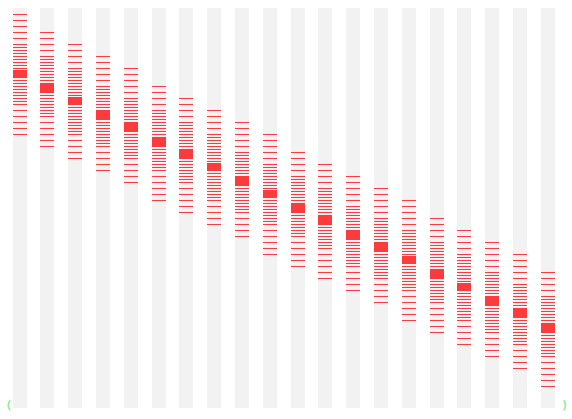
Value encoder. x-axis is numeric range in 5% steps. Active bits vertically.
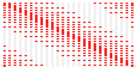
Hour-of-day encoder. x-axis is hour. Active bits vertically.
-
Effective time steps
The time series data in NAB are sampled at different time scales and also change at very different rates. Some are smooth and wavelike and others are super spiky. As I mentioned in the context of the delta anomaly score, sometimes an apparently sharp peak would in fact roll in over many time steps. Because there is only an incremental change on each time step, the magnitude of the anomaly can be underestimated.
The sampling rate at which data happens to be available may not be the best rate for learning meaningful transitions.
One idea is to delay taking an effective time step in HTM until a sufficient change occurs to be registered. That is, wait until the set of active columns are, say, 20% different from the last effective time step. At that point, learn the transitions from the last effective time step.
Interestingly, this gives an improved result on the low FP rate profile:
| model | standard | low FP rate | low FN rate |
|---|---|---|---|
| original NuPIC model + anomaly likelihood | 65.3 | 58.6 | 69.4 |
| original NuPIC model | 52.5 | 41.1 | 58.3 |
| selected Comportex model (above) | 64.6 | 58.8 | 69.6 |
| effective time steps when 20% columns change | 64.7 | 59.8 | 69.5 |
Incidentally, I think the low FP rate profile is the most reasonable. It balances one correctly detected anomaly to about 10 false positives; whereas the standard profile balances one to about 20 false positives, which seems excessive. And low FN rate is more like one to 30.
Limitations
Anyway, this effective time steps approach is interesting but obviously not a final solution. It has no way to detect when an expected event does not occur, since there is no change of value involved.
Ideally I think the system would be entrained to a rhythm according to regular patterns in the data, and that would define effective time steps.
Further work
I’m keen to break down the effects of parameters and algorithm variations by file. Which files change their score order under in each experiment? That could help to investigate what’s going wrong, in detail.
Looking forward to hearing your thoughts directly or on the HTM Forum.
–Felix
-
Code
The results here were produced with nab-comportex 0.1.0 using Comportex 0.0.14.
-
Appendix: Specific experiments
Results here are expressed as a change in score relative to a starting point “baseline” model. The baseline model is the same as headline model except:
- distal stimulus threshold 20
- local receptive field 20% diameter and 80% fraction.
Note: The scoring here is not from official NAB, it is from my own implementation of the NAB scoring rules. And my scores are not quite the same as the official NAB scores, although they are usually closely correlated. I have not tracked down the cause of the inconsistency.
Scores shown as differences from baseline:
|   | settings                                      | standard | low FP rate | low FN rate |
|------------------------------------------------------------------------------------------|
| * | baseline                                      | =0.0     | =0.0        | =0.0        |
|   | without delta anomaly; raw bursting score     | -4.8     | -2.7        | -3.4        |
|   | global receptive field, 80% fraction          | -1.1     | -1.2        | -1.6        |
|   | global receptive field, 16% fraction          | +0.4     | +1.7        | +0.5        |
|   | no timestamp input                            | -3.8     | -3.5        | -3.0        |
|   | depth 32 cells per column                     | -2.6     | -4.6        | -2.3        |
|   | depth 32 cells per column, newly bursting     | -3.2     | -5.9        | -2.3        |
|   | depth 32 cells per column, raw bursting       | -5.5     | -5.8        | -5.7        |
|   | distal stimulus threshold 19                  | +0.3     | +1.0        | +0.8        |
|   | distal stimulus threshold 18                  | +1.1     | +1.5        | +1.9        |
|   | distal stimulus threshold 17                  | -0.1     | +0.9        | +2.0        |
| $ | global receptive field, 16% fraction, stim 18 | +1.3     | +2.5        | +1.4        |
|   | effective time steps when 20% columns change  | -0.8     | +0.5        | -1.3        |
|   | effective time steps when 25% columns change  | -1.9     | +0.1        | -2.4        |
|   | effective time steps when 15% columns change  | -1.3     | -0.7        | -1.5        |
|   | effective time steps, distal stimulus 18      | -0.7     | +1.1        | -0.9        |
| ! | effective time steps, 16% fraction, stim 18   | +1.8     | +3.1        | +2.0        |
|   | depth 32, effective time steps & stimulus 18  | -2.6     | -1.0        | -2.1        |
* baseline model
$ headline model
! headline effective time steps model
Where baseline model scores are (different from official NAB scoring):
|   | settings                                      | standard | low FP rate | low FN rate |
|------------------------------------------------------------------------------------------|
| * | baseline                                      | 66.1     | 60.5        | 70.5        |